You are staring at a price of 1.80 on the cricket side you think is stronger, and someone has told you that expected value in betting is the number that decides whether the stake is worth placing. That is true, but almost every page that says it then skips the actual arithmetic. It defines the idea with a coin flip, declares that positive numbers exist, and spends the rest of its length telling you to go hunting for them. This breakdown does the opposite.
It works the number out three times — on a real-shaped cricket price pair, on a colour prediction round, and on a single casino spin — and shows where the sign of the answer comes from. The short version, before the detail: in every one of those three cases the sign is set by the margin built into the price, and it is set before any opinion, form study or reading of the pitch enters the picture.
Table of Contents
What expected value in betting actually measures
Expected value in betting is the average amount a stake returns or loses per bet, if that exact bet could be repeated an unlimited number of times under identical conditions. It is a long-run average, and it is almost never a result you can actually get on any single bet. A 100-rupee even-money bet either returns 200 or returns nothing; it never returns 97.30. Yet 97.30 is the honest description of what the bet is worth, because that is the figure the average settles on as repetitions pile up.
That gap between the figure and any achievable outcome is the reason the concept is so easy to misread. People hear “expected” and treat it as a prediction. It is not. It is a weighted average of every outcome the bet can produce, each one multiplied by how likely it is. Nothing in the definition says the average will appear soon, or that it will appear in any particular sequence of bets.
Three inputs go into it, and only three: the full list of outcomes, the probability of each outcome, and the money each outcome pays. Get any of the three wrong and the output is worthless. The one that gets fudged most often is the probability — people quietly substitute the price’s implied chance for the real chance, which guarantees a result of zero and hides the margin entirely. The second section below exists specifically to stop that.
It helps to separate two things that often get merged. Expected value tells you the direction and size of the average. Variance tells you how far individual results scatter around it. A bet can have a mildly negative average and still produce long stretches of profit, which is exactly what makes the average hard to notice. If you want the scatter side of the picture in detail, the companion piece on how variance makes short-run results misleading covers the swing arithmetic properly.
The seven calculations, in order
There is no single formula that does the whole job. Working an expectation out from a posted price takes a short chain of steps, and skipping any of them is where most published examples go wrong. Here is the chain, in the order you actually need it.
- Price to implied probability. For a decimal price, divide 1 by the price. A price of 1.80 implies 1 / 1.80 = 0.5556, or 55.56%. This is what the price says, not what is true.
- Add the implied probabilities across the market. For a two-way market at 1.80 and 2.00, that is 0.5556 + 0.5000 = 1.0556. A fair market would total exactly 1.0000. The excess, 0.0556, is the overround.
- Convert the overround into the margin. Divide the excess by the total: 0.0556 / 1.0556 = 0.0526, or 5.26%. That is the slice of every unit staked that the pricing retains on average.
- Normalise to margin-free probabilities. Divide each implied probability by the total. 0.5556 / 1.0556 = 0.5263 and 0.5000 / 1.0556 = 0.4737. These now sum to 1.0000 and are the market’s own view of the real chances, with the margin stripped out.
- Expected value of one stake. Multiply the real probability of winning by the total return on a win, then subtract the stake. On 100 at 1.80 with a real chance of 0.5263: (0.5263 x 180) – 100 = 94.74 – 100 = -5.26.
- Express it per unit staked. Divide the result by the stake: -5.26 / 100 = -5.26%. Per-unit form is the only version worth comparing across bets of different sizes, and it is the number that should go in your records.
- Project it across turnover. Multiply the per-unit figure by total money staked, not by number of bets. Five hundred bets of 100 is 50,000 of turnover, so the projected average loss is 50,000 x 5.26% = 2,630, whatever the win-loss record looks like.
Step four is the one that gets dropped. If you use the price’s raw implied probability at step five instead of the normalised one, the arithmetic returns exactly zero every time, and you conclude the bet is neutral. It is not neutral. The zero is an artefact of feeding the price back into itself.
Step seven is the one people resist, because it detaches the projection from the thing they feel they control. You do not get to choose your loss rate by picking better bets within a priced market; you choose your turnover, and the margin does the rest. Doubling stake size doubles the projected loss without changing the percentage at all.
Two housekeeping notes on the chain. First, it assumes decimal prices throughout. If a price is quoted in fractional form, convert before step one by dividing the numerator by the denominator and adding one, so 4/5 becomes 1.80 and evens becomes 2.00. Second, the chain as written handles a clean two-way market. On a market with three or more outcomes the same steps apply unchanged, except that step two adds every implied probability in the market rather than two of them, and a market with a missing or unquoted outcome cannot be normalised honestly at all, because the total you would divide by is incomplete.
Worked example: a cricket match price pair
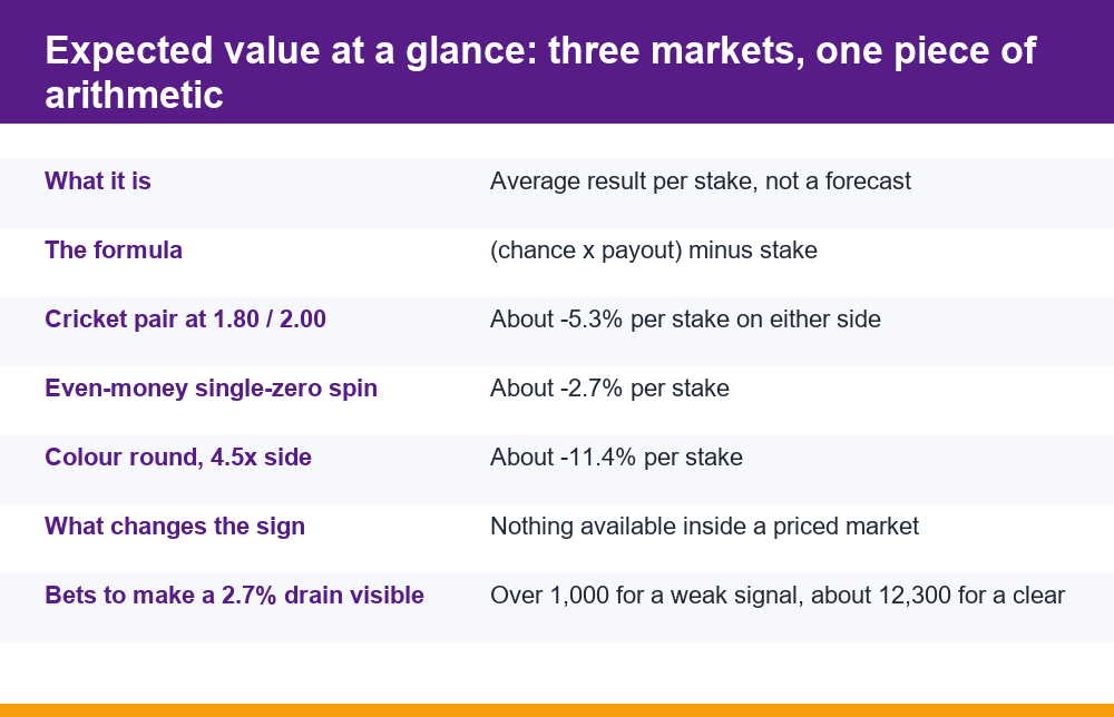
Take a two-way match market priced at 1.80 and 2.00. Run the chain above and the margin comes out at 5.26%, the normalised chances at 52.63% and 47.37%, and the per-stake expectation at -5.26% on either side. That last point is the one worth sitting with: both sides lose at the same rate. There is no favourite-versus-underdog asymmetry here. Backing the side you think is stronger and backing the side you think is weaker produce identical averages, because the margin was spread evenly across the pair when the prices were set.
Now introduce an opinion, purely to see what an opinion is worth in this arithmetic. Suppose you believe, after watching the surface and the team news, that the first side wins 56% of the time rather than 52.63%. Redo step five with your own number: (0.56 x 180) – 100 = 100.80 – 100 = +0.80, or +0.80% per stake. The sign has only just turned, and it has turned on the assumption that your 56% is correct. You moved your estimate 3.4 percentage points away from the market’s and the arithmetic returned less than one percent.
That is the real shape of the problem, and it is the reason this is a demonstration rather than a method: the margin absorbs almost all of any disagreement you can honestly claim to have.
Push the same arithmetic the other way. If your true chance is 50% rather than 56%, the same bet reads (0.50 x 180) – 100 = -10, a 10% average loss, roughly double the market’s own margin. Being six points wrong in your favour gains you almost nothing you would notice; being six points wrong against yourself doubles the damage. Expected value in betting is unforgiving in that direction because the payout is fixed while your error is not.
One more complication that the single-example pages never mention. Prices move. The 1.80 you calculated against may be 1.72 by the time the stake lands, which changes the implied probability to 58.1% and turns a thin positive back into a clear negative. An expectation calculated against a price you did not actually get is not a calculation, it is a memory.
Worked example: one colour prediction round
Colour prediction rounds are structurally simpler than a cricket market and often worse on the numbers. Take a generic round structure, used here purely to illustrate the arithmetic rather than to describe any particular product: ten equally likely outcomes, two colour options each covering five of them and paying 2x the stake, and a third option covering two of the ten and paying 4.5x. Commission of 2% is taken from winnings.
The five-outcome colour: the chance is 5/10 = 0.50. A winning 100 returns 200 gross, and 2% of the 100 profit is withheld, so the net return is 198. Expectation is (0.50 x 198) – 100 = 99 – 100 = -1, or -1% per stake. Tolerable-looking, and that is the point of it.
The two-outcome option: the chance is 2/10 = 0.20, and a winning 100 returns 450 gross, less 2% of the 350 profit, so 443 net. Expectation is (0.20 x 443) – 100 = 88.60 – 100 = -11.40, or -11.40% per stake. Eleven times worse than the option sitting next to it on the same screen, in the same round, on the same outcome.
This is the detail worth taking away, and it is why the mechanic exists in this shape. A product can hold one visible option at a loss rate that looks almost fair while placing a much heavier one directly beside it, labelled only by a bigger multiplier. The multiplier is the advertisement; the probability behind it is not displayed. Neither option is positive, so there is no choice here that turns the round profitable — there is only a choice between a slow drain and a fast one.
A related warning belongs here. Because the underlying probabilities in these rounds are not published and cannot be independently verified by a player, the calculation above is a best case: it assumes the ten outcomes really are equally likely. If they are not, every figure above is too generous. Any arrangement that promises guaranteed returns, recovery of past losses, or a paid signal telling you which colour is next is selling you something that cannot exist, for the simple reason that the sign of the expectation is fixed by the payout table and no outside information changes the payout table.
Worked example: a single roulette spin
A roulette wheel is the cleanest case because the probabilities are a matter of counting pockets rather than estimating form. A single-zero wheel has 37 pockets, 18 of them red. An even-money bet on red wins with probability 18/37 = 0.4865 and returns 200 on a winning 100. Expectation is (0.4865 x 200) – 100 = 97.30 – 100 = -2.70, so -2.70% per stake.
Add a second zero and nothing about the bet changes except the denominator. Thirty-eight pockets, 18 red, so 18/38 = 0.4737. Expectation becomes (0.4737 x 200) – 100 = 94.74 – 100 = -5.26, or -5.26% per stake. One extra pocket nearly doubles the long-run cost of an otherwise identical wager, and the player-facing bet looks exactly the same in both cases.
Notice the number: -5.26%, identical to the cricket pair at 1.80 and 2.00. That is not coincidence, it is the same mechanism showing up twice. A two-way market where the implied probabilities sum to 1.0556 and a 38-pocket wheel paying as though there were 36 are two ways of building the same retained slice. Different surfaces, different vocabulary, one piece of arithmetic. The structural side of this is set out in the breakdown of how the house edge is built into a game’s payout table.
Here are the three worked cases side by side, with per-stake expectation in the final column.
| Bet | Chance of winning | Return on a winning 100 | Expectation per 100 staked |
|---|---|---|---|
| Cricket side priced 1.80 (margin-free chance 52.63%) | 0.5263 | 180 | -5.26 |
| Cricket side priced 2.00 (margin-free chance 47.37%) | 0.4737 | 200 | -5.26 |
| Colour option, 5 of 10 outcomes, 2x less 2% commission | 0.5000 | 198 | -1.00 |
| Colour option, 2 of 10 outcomes, 4.5x less 2% commission | 0.2000 | 443 | -11.40 |
| Even-money bet, 37-pocket wheel | 0.4865 | 200 | -2.70 |
| Even-money bet, 38-pocket wheel | 0.4737 | 200 | -5.26 |
Every row is negative. Not because the examples were picked to be negative, but because in each case the payout was set after the probability was known, by whoever wrote the payout table.
Why the sign is set by the margin before skill enters
This is the part the coin-flip explainers skip, and it is the only part that matters for deciding whether to place a stake. A coin flip paying 2.00 has an expectation of exactly zero: (0.50 x 200) – 100 = 0. Nothing on offer anywhere is priced like that coin flip. Every posted price is the true chance, as estimated by whoever set it, reduced by a slice. The slice is applied first. Your judgement is applied second, to whatever is left.
Written as a single relationship: the expectation per stake equals your estimate of the true chance, multiplied by the payout, minus one. For the sign to be positive, your probability estimate has to be better than the price’s implied probability by more than the margin. Not better than the other side’s view. Not better than the crowd. Better than the price, by more than the retained slice, consistently, after the price has already moved to absorb most public information.
- The margin is charged on turnover, not on losses. It applies to winning bets as well, because it was taken out of the payout before the bet settled.
- It compounds with activity. More bets at the same margin means more turnover, which means a larger projected loss in money even if the percentage never changes.
- It is largely invisible on the screen. A price shows a number, not the slice removed from it. The only way to see the slice is to do steps two and three above.
- It does not depend on which outcome you pick. In an evenly loaded market, every selection carries the same percentage, so no amount of switching sides improves the average.
- Information you have usually is not information the price lacks. Public news, team announcements and form are typically already inside the number by the time you read them.
There is one honest consequence of all this: for the overwhelming majority of people placing the overwhelming majority of bets, the expectation is negative, so loss is the expected outcome rather than an accident. Real-money play carries financial risk and is for adults only. If the arithmetic in this piece is uncomfortable to read against your own record, the independent, non-commercial material on understanding the risks of gambling is a better place to go than another page about finding value. The mechanics of how the slice is inserted into a posted price are set out separately in the piece on how a margin is built into the odds you see.
Why a run of wins does not change the number
Suppose you place twenty even-money bets on a 37-pocket wheel and win thirteen of them. You are up 600 on 2,000 staked, a 30% return. The expectation per stake was -2.70% before you started, and it is -2.70% now. Nothing about the thirteen wins altered the pocket count, the payout or the probability. The arithmetic was never a forecast of those twenty results; it was a statement about the average of an unlimited number of them.
The instinct that fights this is strong, and it runs in both directions. After a winning run, the pull is to conclude that something about your approach is working. After a losing run, the pull is to conclude that a correction is owed. Both conclusions treat independent events as though they remember each other. They do not. Each spin, each round and each settled match starts from the same probabilities as the last one.
It is worth being precise about what independence does and does not mean, because this is where the misreading usually happens. Independence does not say that results even out. It says the opposite: a deficit is never repaid, it is only diluted. If you are 300 behind after a hundred bets, the next hundred bets do not contain a mechanism that returns the 300. They contain their own fresh negative average, and the 300 simply becomes a smaller fraction of a larger total staked. The percentage drifts towards the figure the arithmetic predicted; the money does not come back.
There is also a measurement trap here. If you judge an approach by its recent results, the sample that produced those results is exactly the sample you used to form the judgement, which means the judgement carries all of that sample’s noise. The only honest test is the arithmetic done in advance, from probabilities and payouts, before any results are in. Record the per-stake expectation at the moment the bet is placed and compare the running total of those figures against your actual running total. When they diverge, the actual total is the noisy one.
Expected value in betting is therefore a property of the bet, not of the bettor’s recent history. It is calculable before the event and unchanged by the event. That is what makes it useful for deciding, and useless for explaining what just happened.
How many bets before expected value in betting shows up
Far more than people assume, and the arithmetic is straightforward enough to run here. For a single even-money bet of one unit, the result is either +1 or -1, so the spread of individual results has a standard deviation of roughly 1 unit. Across n independent bets, the cumulative average drifts by about the square root of n units from chance alone, while the systematic drain grows in proportion to n itself.
Set the two against each other. The drain exceeds one standard deviation of noise when the edge multiplied by the square root of n is greater than 1. At a 2.70% edge, that needs the square root of n above 37, so n above about 1,370 bets — and one standard deviation is a weak signal, roughly the point at which the pattern is merely more likely than not. For the drain to stand three standard deviations clear of the noise, you need the square root of n above 111, which is roughly 12,300 bets.
At a 5.26% edge the numbers improve but stay large: about 360 bets for one standard deviation and about 3,250 for three. In other words, a person placing a few bets a week can spend years without the average becoming visible in their own record. Their results will look like skill, or like bad luck, or like nothing in particular, long after the underlying figure has been fixed from the first bet onwards.
Two qualifications keep this from being read as more precise than it is. The figures above assume every bet is the same size and roughly even-money, which keeps the per-bet standard deviation near 1 unit. Mix in longer prices and that spread widens sharply, because a bet that wins one time in five produces much larger individual swings, so the number of bets needed rises rather than falls. And if stake sizes vary, bet count stops being the right unit altogether — the comparison has to be run on turnover, since a handful of large stakes can dominate a long record of small ones and make the average less visible, not more.
This is the most practically important thing on this page, and it cuts against the entire genre of result-based self-assessment. The reason people believe in systems is not that the systems work. It is that the sample needed to disprove one is larger than the sample most people will ever accumulate.
Mistakes that make the calculation meaningless
The chain of seven steps is short, but each step has a characteristic failure, and a single one is enough to turn a careful-looking calculation into a confirmation of whatever you already believed.
- Using implied probability as the real probability. This always returns zero and makes every bet look neutral. Normalise first, or supply your own independent estimate.
- Confusing profit with total return. At a price of 1.80, a winning 100 returns 180 in total, not 180 profit. Mixing the two overstates the expectation by the full stake.
- Leaving commission or deductions out. Anything withheld from winnings belongs inside the payout figure, not noted alongside it.
- Calculating against a price you did not get. Use the price actually struck. A figure based on a better price that has since moved describes a bet nobody placed.
- Ignoring outcomes that are not win or lose. Voids, abandonments, ties and partial settlements are outcomes with probabilities and payouts, and they have to appear in the weighted sum.
- Projecting across bet count instead of turnover. Stake size is what scales the money. Fifty bets of 1,000 and five hundred of 100 carry the same projected loss.
- Treating a recent run as evidence. See the sample-size arithmetic above. A few hundred bets is a rounding error against the number required.
One habit fixes most of these at once: write the expectation down at the moment of placing, in per-unit form, with the price, the probability you used and where that probability came from. The record then contains the reasoning as well as the result, which is the only arrangement in which you can later tell the two apart. Keeping it in money as well as percentages is worth the extra column, because the percentage stays flat while the money tracks how much you actually staked.
None of this produces a way to make the sign positive in a priced market, and nothing on this page should be read as suggesting it does. What it produces is an accurate description of what a stake is worth before it is placed, and an accurate expectation of how long it will take for that worth to become visible. Those two things are the honest content of expected value in betting, and they are usually enough to settle the question of whether a bet is worth placing without any further analysis at all.
Frequently Asked Questions
What is expected value in betting?
It is the average amount a stake returns or loses per bet if that bet were repeated an unlimited number of times under identical conditions. It is built from three inputs: every outcome the bet can produce, the probability of each, and the money each one pays. It is a weighted average, not a prediction, and it is usually a figure no single bet can actually return.
How do you calculate expected value on a bet?
Multiply the real probability of each outcome by the total return that outcome produces, add those products together, then subtract the stake. On 100 at a price of 1.80 with a true chance of 52.63 percent, that is (0.5263 x 180) – 100 = -5.26. Divide by the stake to express it per unit, which gives -5.26 percent. The critical step is using a genuine probability estimate rather than the price’s own implied probability, since feeding the price back into itself always returns zero.
Can expected value be positive for a casino game?
Not for the player on a standard priced game. The payout table is written after the probabilities are known, with a slice retained, so the figure is negative on every available bet. On a 37-pocket wheel an even-money bet averages -2.70 percent per stake and on a 38-pocket wheel it averages -5.26 percent. No sequence of bets, staking pattern or selection of which bet to place within the game changes the sign, because none of those things changes the payout table.
Does expected value tell you what will happen next?
No. It says nothing about the next bet, the next ten or the next hundred. A 100-unit even-money bet with an expectation of -2.70 either returns 200 or returns nothing; it never returns 97.30. The figure describes the centre of a distribution, and individual results scatter widely around that centre. Treating it as a forecast is the single most common misreading of the concept.
Why is expected value negative when odds include a margin?
Because the margin is subtracted from the payout before the bet settles. If a two-way market is priced at 1.80 and 2.00, the implied probabilities sum to 1.0556 rather than 1.0000, and that 5.26 percent excess is retained on average from every unit staked, on winning bets as well as losing ones. For the sign to turn positive your own probability estimate would have to beat the price’s implied probability by more than the margin, consistently, after the price has already absorbed the available public information.
How many bets before expected value shows up?
Many more than most people place. The systematic drain grows in proportion to the number of bets while random scatter grows only with the square root, so at a 2.70 percent edge it takes roughly 1,370 bets for the drain to exceed one standard deviation of noise and roughly 12,300 for it to stand three standard deviations clear. At 5.26 percent those figures fall to about 360 and 3,250. Someone placing a few bets a week can therefore go years without the average becoming visible in their own record.